testing scientific code

In the last post we looked at interactive debugging, a useful tool for expediting the process of getting our code not to crash. But it doesn’t tell us whether our code is actually producing the right results. To verify the correctness of our code, we need to test it, or generate evidence that it’s doing what we expect it to do. This not only brings peace of mind but makes our code easier to modify and extend and more trustworthy in the eyes of others. In this post we’ll go over how to adequately test a codebase, and we’ll see how to implement automated tests in Python and display the results in a Jupyter notebook.

A motivating example

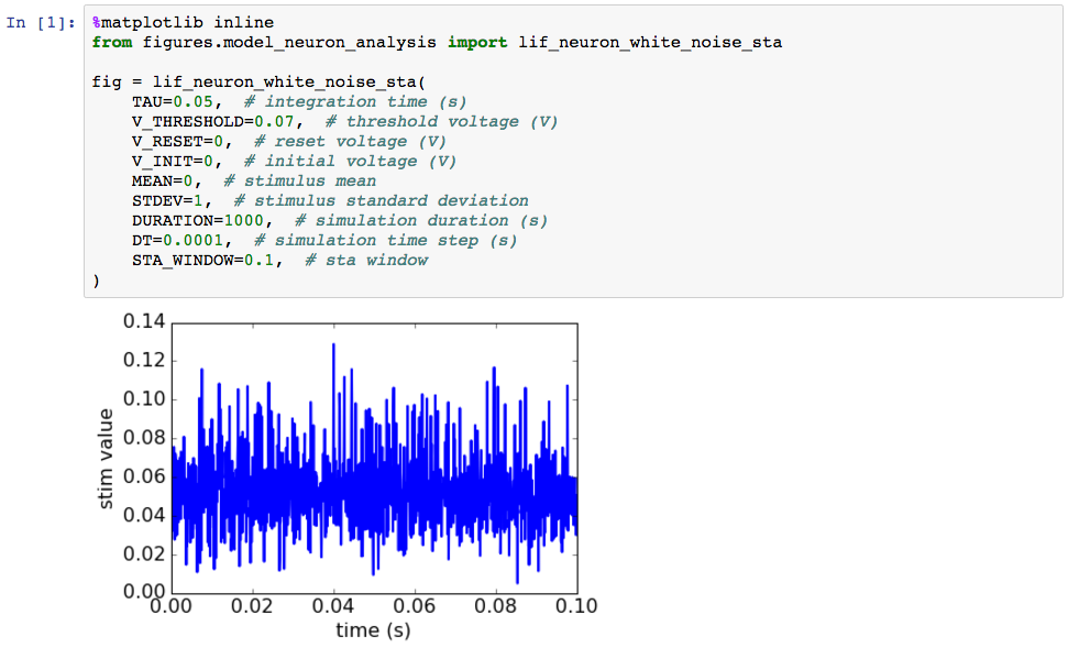
As usual, we’ll draw from an example in neuroscience. The function below attempts to determine the stimulus pattern that makes a model neuron spike (emit an action potential). It does this by presenting a random stimulus to the model neuron, identifying the resulting spikes, collecting the stimuli over a short window of time preceding each spike, and then averaging these over the spikes to generate the spike-triggered average (STA). While this is a relatively straightforward procedure, it is complex enough that there is a good chance something can go wrong even if the code doesn’t crash. As before we’ll call the function we’ve written to do this from inside a Jupyter notebook cell:

As we can see, our function call produced a plot and didn’t throw an error, so that’s a good start. And we see that the resulting STA is a current that generally maintains a positive value over the time window preceding the spike. Since positive current inputs are supposed to make neurons spike, this seems ostensibly reasonable. But can we trust the result? To find out we need to write some tests.

Identifying code components

The question before us now is: what tests will provide the strongest evidence that our code is working correctly? And fortunately, the general answer is straightforward. We simply need to identify the components of our code that have a known, expected behavior under certain conditions, and then ensure that these in fact behave as expected under said conditions.

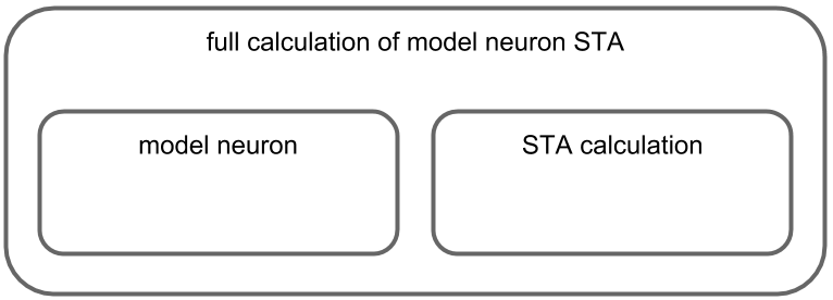
The first step, then, is to identify the “natural” components of our code. In the present case this is quite easy, since there’s a fairly clear hierarchical organization. The outermost component is the function we’ve called inside the notebook cell, and this component is itself composed of two smaller components: the model neuron that generates the spike sequence and the computation of the STA.

Note, however, that partitioning a more complex codebase into sensible components might require a bit more thought. Still, it is worth putting in the effort, as a clearly organized codebase makes not only testing it but interacting with it in general quite a bit easier.

Deciding which components to test and how to test them

Next we need to figure out which of these components to test and how to test them. One approach I’ve found to work well has been to start from the outermost, or top-level component and then work inwards. This is because if the top-level component works there’s a good chance the smaller components work, whereas the reverse is less probable.

In our case, the top-level component is the function we called inside the notebook cell, i.e., the full calculation of the model neuron’s STA. To see if we can test this component in a meaningful way we need to try to find a set of conditions (i.e., arguments passed to the function) under which we know exactly what behavior to expect. That is, are there any sets of arguments for which the true STA is already known?

As it turns out, this analysis has actually been published, so in reality we do have something to compare our top-level results to. However, while scouring the literature for similar ideas is always highly recommended when doing an analysis of one’s own, today we’re going to pretend that we don’t have access to any sort of “ground truth” results for the top-level component. This is often the case when performing an original computation and in fact often the reason you’re performing said computation in the first place. What this means is that testing our top-level function is going to be rather fruitless, since we won’t have any way to judge the results. Instead we’ll have to satisfy ourselves with testing the lower-level components. And this is completely fine: if they both work exactly as expected, then we can still argue that the top-level component works also, since it is a simple combination of the two.

Fortunately, we do have some idea about how the model neuron should behave, and this can help us design our tests. First, it should produce no spikes when provided with an input current of zero. Second, the spike rate should increase as the input current increases. Third, the spike rate should increase as the neuron’s threshold decreases.

How can we test the STA computation? Well, first we know that if the spikes are independent of the current, the STA should be near zero. Second, if each spike is preceded precisely by a short, stereotyped stimulus, then the STA should recover that stimulus. Scientifically speaking, the first test is akin to a negative and the second to a positive control.

Note that this is again one of those aspects of testing that requires some thought. When deciding which tests to write, we must ask ourselves which behaviors each component of our code must produce to convince us that it is working correctly, and this is highly dependent on the details. In general, while more tests never hurt, I’ve found it much more satisfying to have a few really convincing tests than a bunch of minor ones.

Anyway, we’ve made some tangible progress now. We’ve got a list of things the model neuron should do if it works correctly and we’ve got a list of the things the STA computation should do if it works correctly. And as I said, that was the hard part. Now all that we have to do is implement them.

Implementing automated tests in Python

Below are the three files (besides the notebook) that we used to perform our full analysis. The first is the the figures module containing the function to run the simulation, compute the STA, and make the plot, and the second is a module containing the model neuron class and third is a module containing the STA computation function. While we don’t necessarily need three separate files for this small example, this is how you might organize your code in a more involved project investigating additional model neuron types and computations.

# contents of model_neurons.py
import numpy as np


class LIFNeuron(object):
    """
    Class for model neuron of the integrate-and-fire variety.
    """

    def __init__(self, tau, v_threshold, v_reset):

        self.tau = tau
        self.v_threshold = v_threshold
        self.v_reset = v_reset

    def run(self, stim, v_init, dt):
        """
        Record the response of the neuron to a stimulus.

        :param stim: 1D array of injected current values
        :param v_init: starting voltage
        :param dt: simulation time step
        """

        n_steps = len(stim)

        vs = np.nan * np.zeros((n_steps + 1,))
        spikes = np.zeros((n_steps + 1,), dtype=int)

        # set initial voltage and spiking state

        vs[0] = v_init
        spikes[0] = int(v_init >= self.v_threshold)

        # loop over all stimulus values

        for step in range(n_steps):
            
            # implement standard voltage-updating equation
            
            dv = (dt / self.tau) * (-vs[step] + stim[step])
            v_next = vs[step] + dv

            # make neuron spike if voltage is above threshold
            
            if v_next > self.v_threshold:
                
                # increase to spike voltage at this time step
                
                vs[step] = self.v_threshold + (self.v_threshold - self.v_reset)
                
                # reset voltage and record spike
                
                v_next = self.v_reset
                spikes[step] = 1

            vs[step + 1] = v_next

        return spikes

# contents of spike_train_analysis.py
import numpy as np


def compute_sta(stim, spikes, window_len):
    """
    Compute the spike-triggered average from a stimulus and a spike train.

    :param stim: stimulus vector
    :param spikes: spike train vector (same len as stim)
    :param window_len: number of time steps in STA window
    """

    n_spikes = int(spikes[window_len:].sum())
    spike_times = window_len + spikes[window_len:].nonzero()[0]

    stims_preceding = np.nan * np.zeros((n_spikes, window_len))

    for spike_ctr, spike_time in enumerate(spike_times):

        stims_preceding[spike_ctr, :] = stim[spike_time - window_len:spike_time]

    # calculate spike-triggered average

    sta = stims_preceding.mean(axis=1)

    return sta

# contents of figures/model_neuron_analysis.py
import matplotlib.pyplot as plt
import numpy as np

from model_neurons import LIFNeuron
from spike_train_analysis import compute_sta


def lif_neuron_white_noise_sta(
        TAU, V_THRESHOLD, V_RESET, V_INIT,
        MEAN, STDEV, DURATION, DT,
        STA_WINDOW):
    """
    Calculate the STA for a leaky integrate-and-fire neuron.
    """

    # make stimulus

    n_steps = int(DURATION / DT)
    stim = MEAN + np.random.normal(0, STDEV, n_steps)

    # make neuron and drive it with stim

    neuron = LIFNeuron(tau=TAU, v_threshold=V_THRESHOLD, v_reset=V_RESET)
    spikes = neuron.run(stim=stim, v_init=V_INIT, dt=DT)

    # compute STA

    n_steps_window = int(STA_WINDOW / DT)
    sta = compute_sta(stim=stim, spikes=spikes, window_len=n_steps_window)

    # make time vector

    t = np.linspace(0, STA_WINDOW, len(sta))

    # plot STA

    fig, ax = plt.subplots(1, 1)

    ax.plot(t, sta, lw=2)
    ax.set_xlim(0, STA_WINDOW)
    ax.set_xlabel('time (s)')
    ax.set_ylabel('stim value')

    # increase fontsize for all text elements
    
    for text in [ax.title, ax.xaxis.label, ax.yaxis.label] + \
        ax.get_xticklabels() + ax.get_yticklabels():

        text.set_fontsize(16)

    return fig

We’ll now make two more files to write and run our tests. The first we’ll call test_model_neuron_analysis.py, and we’ll put it inside a new directory called “tests”. The second will be the notebook in which we run the tests, which we’ll call “tests.ipynb”. Our final directory structure looks like this.

.
|-- model_neurons.py
|-- spike_train_analysis.py
|-- figures
    |-- model_neuron_analysis.py
|-- analysis.ipynb
|-- tests
    |-- test_model_neuron_analysis.py
|-- test.ipynb

The testing framework we’ll be using is called pytest. While it is not the only framework available, it requires minimal boilerplate code and is simple to use. Each of the tests we decided upon in the previous section will be contained inside a single function within the file test_model_neuron_analysis.py. Each function name should start with “test” and provide as specific as possible a description of what the test does. For example, a good name for the first test of our model neuron component would be “test_neuron_produces_no_spikes_given_zero_input”. Inside this testing function we’ll create a model neuron, drive it with a zero-valued stimulus, and count the number of spikes in the resulting spike train. Next we’ll implement the most important part of the test, without which the function wouldn’t be a test at all. That is, we will now use the assert keyword to ensure that the number of spikes in the spike train is zero. The only rule about the assert keyword is that it must be followed by a statement that evaluates to a truth value. The full test looks like this.

def test_lif_neuron_produces_no_spikes_given_zero_input():

    import numpy as np
    from model_neurons import LIFNeuron

    # make model neuron and zero-valued stimulus

    neuron = LIFNeuron(tau=0.05, v_threshold=0.07, v_reset=0)
    stim = np.zeros((50000,))

    # present stimulus to neuron and count spikes

    spikes = neuron.run(stim, v_init=0, dt=0.0001)
    n_spikes = spikes.sum()

    # make sure there are zero spikes

    assert n_spikes == 0

One other important thing to note is that each test should be completely self-contained. That is, no test should rely on the results of other tests. This way they can all be run independently. Additionally, test names should be very descriptive so that a user can figure out what’s being tested as quickly as possible. This is one of the times when typical style rules about maximum line length can be ignored. These tests are fairly simple, but if they can’t be completely described in the title they should contain an accompanying docstring describing what they’re testing in more detail.

When we have written all three of the tests for the model neuron component of our analysis, the file test_model_neuron_analysis.py will contain the following.

# model neuron tests

def test_lif_neuron_produces_no_spikes_given_zero_input():

    import numpy as np
    from model_neurons import LIFNeuron

    # make model neuron and zero-valued stimulus

    neuron = LIFNeuron(tau=0.05, v_threshold=0.07, v_reset=0)
    stim = np.zeros((50000,))

    # present stimulus to neuron and count spikes

    spikes = neuron.run(stim, v_init=0, dt=0.0001)
    n_spikes = spikes.sum()

    # make sure there are zero spikes

    assert n_spikes == 0


def test_lif_neuron_spike_rate_increases_as_input_increases():

    import numpy as np
    from model_neurons import LIFNeuron

    # make model neuron

    neuron = LIFNeuron(tau=0.05, v_threshold=0.07, v_reset=0)

    # make several stimuli with increasing means

    stims = [np.random.normal(0.5*ctr, 1, 50000) for ctr in range(10)]

    # run neuron for each stimulus and count spikes

    spikes_all = [neuron.run(stim, v_init=0, dt=0.0001) for stim in stims]
    n_spikes_all = [spikes.sum() for spikes in spikes_all]

    for n_spikes_prev, n_spikes_next in zip(n_spikes_all[:-1], n_spikes_all[1:]):

        assert n_spikes_prev < n_spikes_next


def test_lif_neuron_spike_rate_increases_as_threshold_decreases():

    import numpy as np
    from model_neurons import LIFNeuron

    # make stim

    stim = np.random.normal(0, 1, 50000)

    # make model neurons

    v_thresholds = [0.08, 0.07, 0.06, 0.05, 0.04]
    neurons = [
        LIFNeuron(tau=0.05, v_threshold=v_threshold, v_reset=0)
        for v_threshold in v_thresholds
    ]

    # run each neuron for stimulus and count spike

    spikes_all = [neuron.run(stim, v_init=0, dt=0.0001) for neuron in neurons]
    n_spikes_all = [spikes.sum() for spikes in spikes_all]

    for n_spikes_prev, n_spikes_next in zip(n_spikes_all[:-1], n_spikes_all[1:]):

        assert n_spikes_prev < n_spikes_next

Next we will run these three tests inside the Jupyter notebook “tests.ipynb”. Again, this is quite simple. We need only one cell containing the following lines.

In fact, within this cell is the only place we actually need to reference pytest. The second line says to look for tests in the directory “tests”. When we run the cell we get the following output.

The output tells us that one test file was found, called “test_model_neuron_analysis.py” and that all three of our tests passed. So far, so good. Now let’s write the tests for the STA computation. These should look something like this and should go in the second half of the file “test_model_neuron_analysis.py”.

# STA computation tests

def test_sta_is_near_zero_when_spikes_are_independent_of_stimulus():

    import numpy as np
    from spike_train_analysis import compute_sta

    # make random stim

    stim = np.random.normal(0, 1, 50000)

    # make random spikes

    spikes = np.random.rand(50000) < 0.05

    sta = compute_sta(stim, spikes, 1000)

    # make sure STA is sufficiently close to zero

    assert np.abs(sta.mean()) < 0.01


def test_sta_recovered_when_all_spikes_preceded_by_same_stim():

    import numpy as np
    from spike_train_analysis import compute_sta

    # make true sta and line it up with several spikes

    n_steps_sta = 500
    sta_true = np.exp(np.arange(-n_steps_sta, 0)/100.)

    stim = np.zeros((50000,))
    spikes = np.zeros((50000,))
    spike_idxs = [1000, 2000, 5000, 10000, 20000, 40000]

    for spike_idx in spike_idxs:
        
        # place the true STA in the window just before the spike
        
        stim[spike_idx-len(sta_true):spike_idx] = sta_true
        spikes[spike_idx] = 1

    sta = compute_sta(stim, spikes, n_steps_sta)

    # make sure difference between computed and true STA is basically zero

    assert round(np.sum(np.abs(sta - sta_true)), 7) == 0

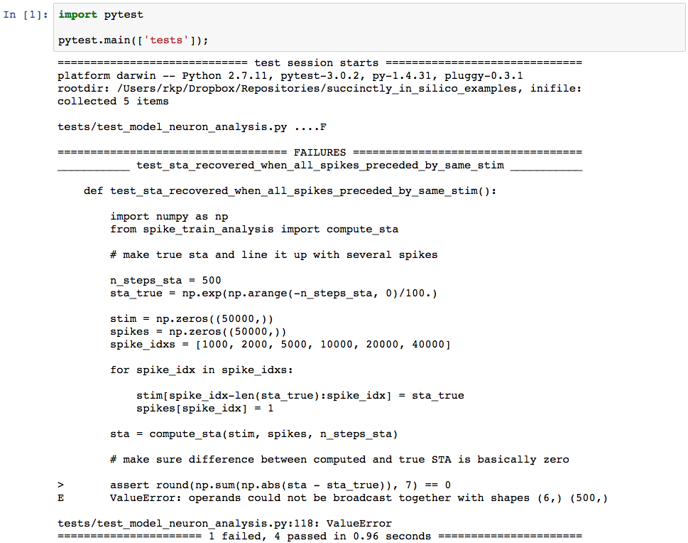
When we go back to our testing notebook to run the new tests we get the following output.

Uh oh. It looks like something went wrong. The testing output tells us that test_sta_recovered_when_all_spikes_preceded_by_same_stim has failed. This means that this whole time our code was producing incorrect results, in spite of the fact that it never threw an error. And if we hadn’t tested it we might never have realized it. I won’t go into the details of the best methods for narrowing exactly how and where an error has occurred, but in this case it turns out that the error was in second to last line in the function sta_computation in the file spike_train_analysis.py in our root directory. Specifically, we had performed the averaging over the wrong axis. When we correct the faulty line

sta = stims_preceding.mean(axis=1)

to

sta = stims_preceding.mean(axis=0)

and run our tests again we get the following output.

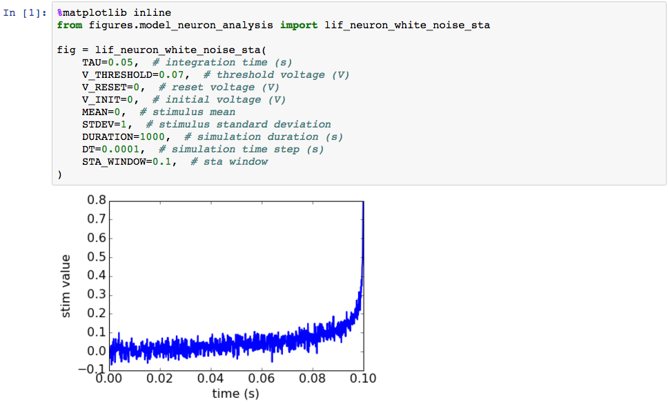
And indeed, our tests have passed. When we run our original plot-producing function we now see the following, which is quite different from the original output.

To an untrained eye this plot might not immediately look any more correct than the original output of the malfunctioning code, but since we have tested the major components of the code used to create it, the result has become significantly more trustworthy.

Final thoughts

My goals in this post were (1) to point out that testing is useful, since functions that don’t throw errors can still produce incorrect results, and (2) to show how to apply a basic Python testing framework (pytest) to scientific code. That said, there’s a lot I haven’t covered here (as well as a lot I have yet to learn myself). Most notably, while our example was intended to provide a feel for the general principles involved, I didn’t go into much detail regarding choosing which tests to write for which components of your code. The main reason for this was that although such details have been largely worked out for the development of commercial software, one would be hard pressed to say the same about scientific code. Some principles carry over from the commercial side, such as testing general use cases for each code component, but some principles are less important, such as testing your code against all possible inputs a user could create by banging on the keyboard. I’ll reiterate, however, that one thing I’ve found useful when testing scientific code is to think in terms of controls (in the scientific sense): a good test suite should contain what amount to a reasonable set of negative and positive controls for each component of your code base. When we tested the function compute_sta, for example, the negative control showed that the STA was close to zero when the spikes were random with regard to the stimulus, and the positive control showed that when the same brief stimulus preceded each spike, the recovered STA would be equal to that stimulus. For other projects, however, the most useful controls to test may be completely different. The only overarching guideline to keep in mind is that the primary goal of testing is to provide good evidence that your code is doing what it’s supposed to do (which will in turn make your code more organized, easier to extend, etc.). The rest is really project-specific thoughtfulness and a little bit of art, both of which speak to the fact that testing is at least to some extent a scientific and creative process.

Additionally, it can be easy to think that it’s just not worth the time to write tests, especially since tests can end up being over half of your entire codebase. While this is somewhat of a fair point, since it’s possible to waste time writing tests that aren’t useful, a good set of tests should in fact save you time in the long run. For instance, let’s say we want to optimize the function compute_sta to keep a running average of the spike-triggering stimuli as it loops through spikes, instead of storing them all in a matrix and averaging at the end. Since we’ve already written our tests for compute_sta, all we have to do after modifying the function is to run them again in our testing notebook, and we’ll know immediately if we’ve modified the function correctly. Further, most scientific coders are in fact testing their code at least to some extent as they write it, running snippets of code in an interpreter to make sure their matrices are getting reshaped correctly, making sure their results look reasonable with respect to what they know from the literature, etc. The only difference here is that we’re writing our tests in a principled way and saving and organizing them so that we can run all the tests every time we modify any aspect of our code, so in theory it shouldn’t require much more effort.

In conclusion, I just wanted to share some of the reasons that testing scientific code as we’ve described above is not only worthwhile, but relatively straightforward to do in a principled and automated way. I hope you’ve found some of my words useful and would be happy to hear any and all of your comments.